The Cassini/MIMI Science Planning and Visualization Tool
Abstract
JCSN is a science planning and visualization tool for the MIMI instrument on the Cassini orbiter. It can be used to view spacecraft attitude relative to various bodies in the Saturnian system. It is also useful for displaying the MIMI instrument sensor fields of view, which provide a simple, visual flight rule constraint checker to find optimum pointing.
The JCSN User's Guide is currently incomplete, and should be considered a work in progress. The plots section is still being written, and the contents of the current release have yet to undergo any serious review. Please feel free to direct comments, questions and concerns to MIMI Webmaster, though they may already be addressed in an updated, yet-to-be-released version of this guide.
Table of Contents
List of Figures
- 1. Sample JCSN Session
- 2. Orbit Selection Controls
- 3. Time Functions Panel
- 4. Spacecraft Attitude Panel
- 5. An Example Plot Panel
- 6. Plot Save Dialog
- 7. Plot Print Dialog
- 8. Time Selection and the VCR Style Controls
- 9. Orbit Browser
- 10. Saturn-Cassini Distance
- 11. Cassini Trajectory XY Overview (SSO)
- 12. Saturn Moon Encounter XY (RTN)
- 13. Saturn Moon-Cassini Distance
- 14. The Visualization Options Window
- 15. Rendering the Sun Line
- 16. Rendering the Sun Shade
- 17. Titan Trajectory Trace
- 18. Selecting the Spacecraft Attitude Model
- 19. PDT Pointing Model Interface
- 20. Body Axis Controls
- 21. “RA and DEC” Controls
- 22. “Vector” Controls
- 23. Target Selection Controls
- 24. “EME 2000” Target
- 25. Limb Target
- 26. Limb Targeting Geometry
- 27. Supplemental Attitude Controls
- 28. Euler Rotation Model Interface
- 29. Euler Angle Configuration
- 30. C-kernel Model Interface
- 31. The “Load C-kernel” Dialog
- 32. The “Unable to Load C-kernel” Dialog
- 33. The Button
- 34. Reconstructed Attitude Dropout
- 35. Reconstructed Data Supplemented with Predict
- 36. C-kernel Attitude History Missing Source Data
- 37. C-kernel Attitude History Predict Only Source Data
- 38. C-kernel Attitude History Reconstructed Source Data
- 39. Sun, Saturn, and Cassini
- 40. Saturn, Reference Moon, and Cassini
- 41. Saturn and Cassini
- 42. Saturn Solar Orbit (SSO) Configuration
- 43. Saturn Equatorial System (SZS) Configuration
- 44. Corotation Configuration
- 45. Saturn Moon System (SZM) Configuration
JCSN is a science planning and visualization tool for the MIMI instrument on the Cassini satellite. It displays a wide variety of quantities useful for constraint checking and pointing optimization. These include spacecraft orientation relative to various bodies and physical quantites of interest in the Saturnian system. It provides a facility for overlaying the sensor's fields of view on skymaps presented in different frames of interest.
Throughout this guide, documentation that appears outside of the normal discussion flow will be marked off from the remainder of the text. The purpose of each of these sections is denoted by the particular markings utilized. They are summarized briefly below:
![[Tip]](gfx/admonitions/tip.gif) | |
Additional information that may be useful and not obvious from the discussion at hand. |
![[Note]](gfx/admonitions/note.gif) | |
A parenthetical comment containing information pertinent to the discussion, but not necessarily related directly. |
![[Caution]](gfx/admonitions/caution.gif) | |
A cautionary remark that is set off to indicate it should be read or considered carefully. |
![[Warning]](gfx/admonitions/warning.gif) | |
A warning that provides information about a component of JCSN that is “fragile” or a discussion of inputs that may violate assumptions the application makes. |
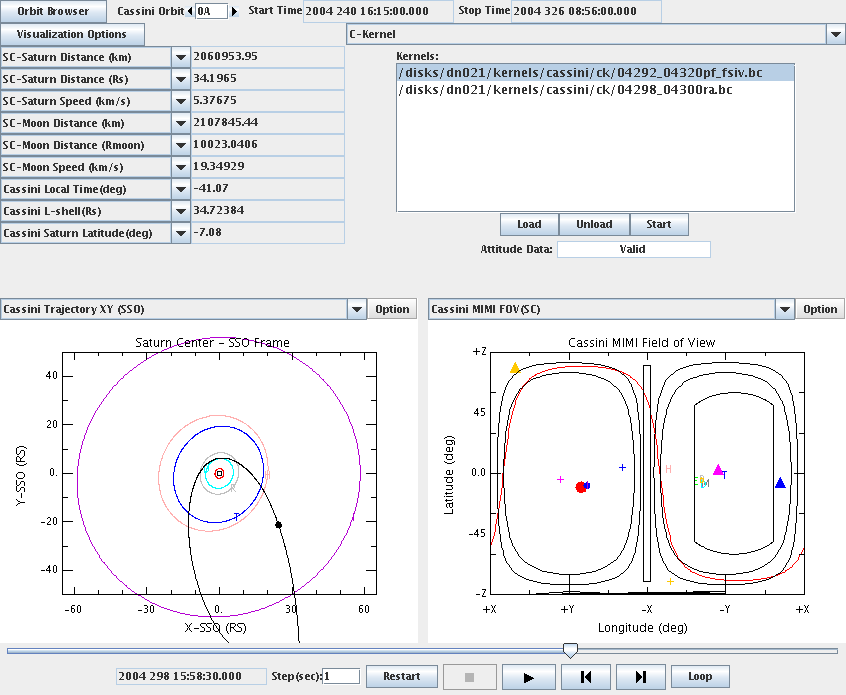
This document describes all of the program options, displays, user controls, coordinate systems, assumptions, and models available within the program. A sample JCSN session is displayed in Figure 1, “Sample JCSN Session”.
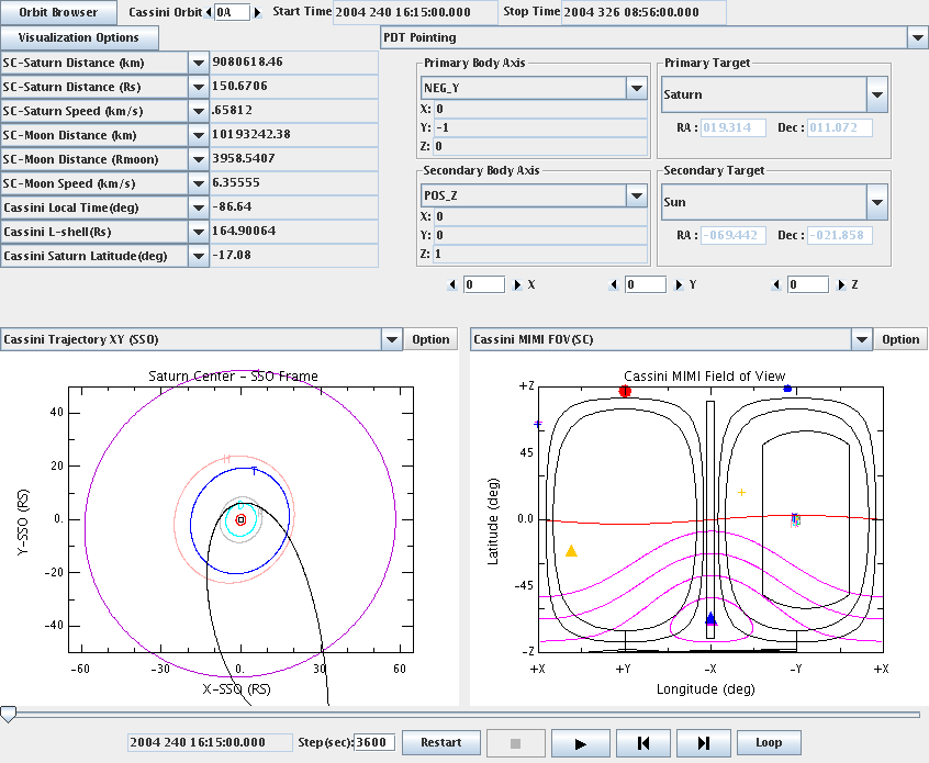
The main JCSN window can be divided into several distinct functional groups. The following sections will discuss these groups, their purpose, and content.
The user controls for JCSN are presented on three separate windows: the main window, the orbit browser, and the visualization options window. This section addresses their purpose and function.
JCSN's application window can be subdivided into several distinct functional groups: the orbit selector, time functions, spacecraft attitude control, plots, and the time selector. Each of these provides a different set of controls to adjust the content displayed.
JCSN presents visualization data on a per orbit basis. The orbit selection controls are located at the top of the main window, as illustrated in Figure 2, “Orbit Selection Controls”.

The orbit number can be entered into the text field directly by clicking in the box, replacing the displayed number with the one of interest and pressing Enter. Clicking the arrows on either side of the text box will increment or decrement the currently displayed orbit number by one. Lastly, the orbit can be specified by interacting with the orbit browser. Click the button to open the orbit browser. See Section 3.2, “The Orbit Browser” for details. Once an orbit is selected, the start and stop times located directly to the right of the orbit selection text box are updated to reflect the chosen orbit.
| |
Neglecting to press Enter after changing the orbit number in the text box will result in the update of the displayed value, but not the value JCSN is currently using. |
The time functions section of the display is located on the left portion of the JCSN window, just underneath the orbit selection controls. This section of the window provides the values of several functions computed at the time currently displayed in the application. Figure 3, “Time Functions Panel” illustrates the default state of the time functions portion of the window:
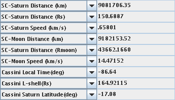
To change the list of time functions displayed, simply click the combo box on the function to replace and select the new function from the presented list. For details on the available time functions, see Section 5, “Time Functions”.
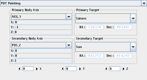
Just below the orbit selection controls and to the right of the time functions are the spacecraft attitude model controls. This portion of the window allows the selection and the adjustment of the model JCSN uses to determine spacecraft orientation with respect to other frames. There are several models available, see Section 4, “Spacecraft Attitude Models” for a detailed discussion. Figure 4, “Spacecraft Attitude Panel” illustrates the PDT pointing model and its controls:
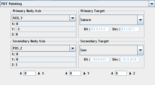
Note the combo box at the top of the panel. This allows the selection of the spacecraft pointing model. Once a particular model is selected, the contents of the panel underneath change enabling customizations or settings specific to the selected model. When a new model is chosen it immediately begins providing JCSN with spacecraft attitude.
There are two customizable plot panels near the bottom of the JCSN window just above the time selection controls. These two windows provide access to a library of available plots. A sample is shown in Figure 5, “An Example Plot Panel”.
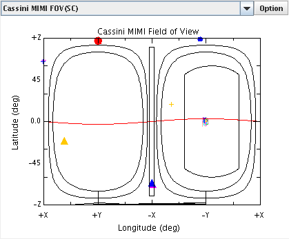
The combo box at the top of the panel selects the plot for display from the library of supported plot types. See Section 6, “Plots” for details. Clicking to the right of the combo box opens a menu with three choices:
The Plot Option Menu
- Help
Currently an unimplemented feature of JCSN. In the future, this will open a help dialog providing information specific to the corresponding plot.
- Save Plot as
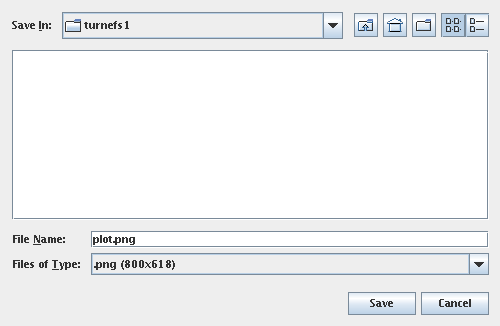
This option opens the Save dialog box show in Figure 6, “Plot Save Dialog”.
To save the plot, use the combo box at the bottom of the window to select from among the available output types, enter the desired filename into the “File Name” text box, then click .
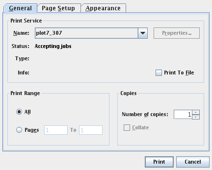
This option opens the Print dialog box. This dialog box varies from platform to platform. Figure 7, “Plot Print Dialog” illustrates the dialog on Linux.
After choosing the appropriate options, clicking will send the image to the selected printer.
At the bottom of the window lie the time selection and playback controls. This interface is used to specify the currently displayed time within the selected orbit. The interface, illustrated in Figure 8, “Time Selection and the VCR Style Controls”, consists of a slider, a text box for specifying the step size, and a collection of VCR style controls.

Dragging the slider adjusts the displayed time within the currently selected orbit. Underneath the slider lie the remainder of the interface controls. From left to right, the first text box encountered illustrates the currently displayed time in JCSN. Next, a text box which permits the specification of the step size in seconds. To adjust the step size, click in the box, replace the time with a new step size, and then hit the Enter to activate it. The step size is the parameter JCSN uses to determine what change in time to use when updating the display with the VCR controls.
| |
Changing the step size, but neglecting to hit Enter will result in the new, updated stepsize's display. However, JCSN will not actually update the utilized stepsize until Enter is pressed. Thus, the VCR controls will respond as if no change has been made. |
Immediately following the step size text box are the VCR style controls. Clicking resets the time to the start of the selected orbit. Just to the right of are and . These buttons function just like the controls on a VCR. Clicking starts JCSN moving forward in time, updating the display once per step size. Most of the user interface controls in JCSN are disabled in this animation mode. Clicking halts the playback, and restores the interactive state of the interface.
After the and are and buttons. When not in animation mode, these buttons can be used to nudge JCSN's currently selected time back or forward a single step size. Lastly, clicking will place JCSN into an animation state where it continues looping over the entire selected orbit until is clicked.
The orbit browser provides an additional, independent mechanism for selecting the active orbit in the JCSN main window. To open the browser window, click the button at the top of the JCSN main window. A new window opens, as illustrated in Figure 9, “Orbit Browser”.
The contents consist of a set of controls to adjust the orbit, a plot window similar to those presented in the main JCSN window, and lastly a set of buttons to commit the currently selected orbit in the browser back to JCSN.
At the very top of the window, there is an orbit selection text box surrounded by arrows. Clicking the arrows adjusts the orbit displayed in the browser window incrementally. Clicking in the text box, replacing the existing orbit with another valid orbit, and pressing Enter on the keyboard also changes the currently displayed orbit.
| |
Neglecting to hit Enter after manually changing the orbit number in the text box will result in the update of the display, but not the value the orbit browser is currently using. |
Following the orbit selection interface is a combo box which adjusts the reference moon. The selected reference moon is used by the plot panel to produce any of the moon based plots.
The plot panel has precisely the same set of controls as the panels in the main JCSN window. See Section 3.1.4, “Plots” for details.
Orbit Browser Supported Plot Types
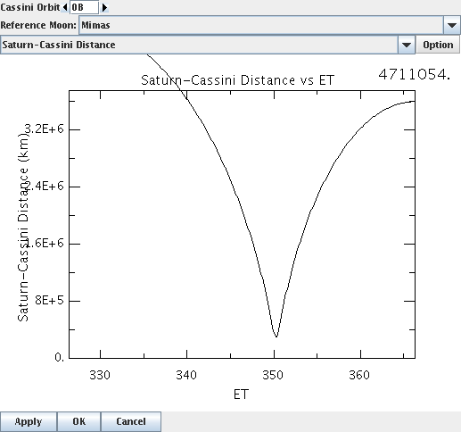
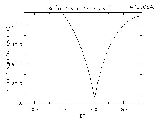
- Saturn-Cassini Distance
This plot presents the distance between Cassini and Saturn expressed in kilometers as a function of the time throughout the currently selected orbit. An example is shown in Figure 10, “Saturn-Cassini Distance”. The number in the upper right corner is the actual distance between Cassini and Saturn at the start of the plot.
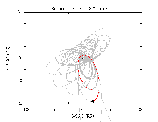
- Cassini Trajectory XY Overview (SSO)
This plot illustrates the entire Cassini mission trajectory relative to Saturn in the Saturn Solar Orbit (SSO) frame. A sample is presented in Figure 11, “Cassini Trajectory XY Overview (SSO)”. The projection of the trajectory onto the XY plane of this frame is show in grey. The small circle at the center of the plot is Saturn, and the orbit highlighted in red is the currently selected orbit. See Section 7.4, “Saturn Solar Orbit (SSO) Frame” for a detailed discussion of this reference frame.
After clicking on the plot within the orbit browser window, the Up Arrow and Down Arrow keys may be used to zoom the view in and out, respectively.
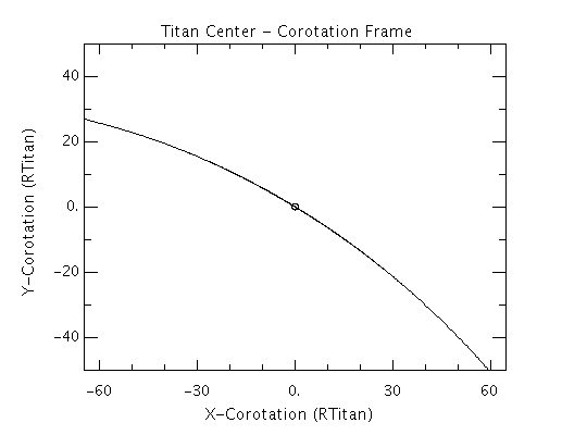
- Saturn Moon Encounter XY (RTN)
This particular plot presents the spacecraft trajectory in the XY plane of the Corotation frame for the currently selected moon. The circle in the center of the plot is the outline of the moon. The black line is the spacecraft trajectory projected onto the XY plane of the Corotation frame. Figure 12, “Saturn Moon Encounter XY (RTN)” shows a sample of a Titan encounter. See Section 7.6, “Corotation Frame (RTN)” for a detailed discussion of the Corotation frame.
After clicking on the plot within the orbit browser window, the Up Arrow and Down Arrow keys may be used to zoom the view in and out, respectively.
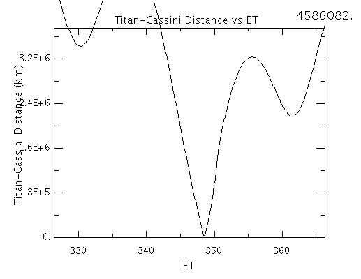
- Saturn Moon-Cassini Distance
This plot gives the distance between Cassini and the currently selected reference moon in kilometers as a function of time throughout the selected orbit. A sample, with Titan as the reference moon, is displayed in Figure 13, “Saturn Moon-Cassini Distance”. The number in the upper right corner is the actual distance between Cassini and Titan at the start of the plot.
At the bottom of the orbit browser window are three buttons used to communicate the selected orbit to the JCSN main window. Click to set the orbit in the main window to the orbit selected in the browser. This will close the orbit browser window. Click to apply the selected orbit to the JCSN main window, but leave the orbit browser window open. Lastly click to close the orbit browser window without changing the orbit selection in the main window.
| |
The selection of the reference moon in the orbit browser only impacts the plots displayed in the orbit browser window itself. Clicking or only commits the selected orbit to the JCSN main window. To change the reference moon in the main window, see Section 3.3, “Visualization Options”. |
The visualization options window provides a set of controls to customize the information displayed in the time functions and plot panels present in the main JCSN window. To access the window, click the button just underneath the orbit selection controls. A window opens, as illustrated in Figure 14, “The Visualization Options Window”.
A detailed discussion of each control and its function follow. Each option changed here takes effect immediately.
| |
Some of the more computationally intensive functions, such as the body tracers, may seem to stall the JCSN user interface while their evaluation completes. |
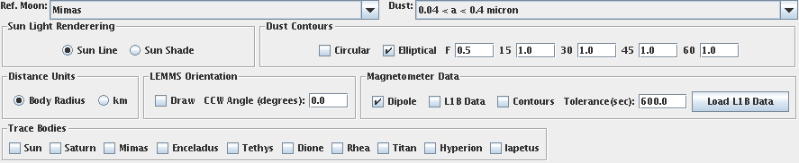
Visualization Options
- Reference Moon
Every JCSN session has a reference moon that is used to support computations for a handful of plots and time functions displayed in the main window. The “Ref. Moon” combo box allows the selection of this moon. Changing the value in the box results in the immediate update of the information in the JCSN main window.
- Dust Particle Size
Some of the plots depend on evaluating a dust model for a particular range of particle sizes. The “Dust” combo box presents a selection of ranges that can be used. Changing the selected range results in an immediate update of any components in the main JCSN window dependent on this range.
- Sun Light Rendering
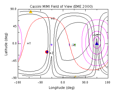
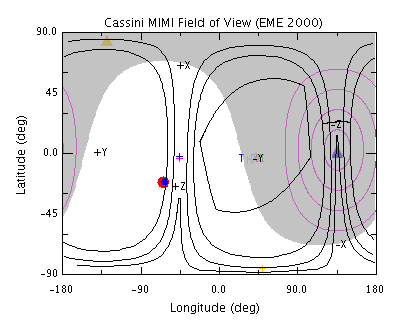
The two radio buttons presented here control how the sun light rendering is performed in the field of view based plots. If “Sun Line” is selected, then a simple red line is drawn to express the boundary between night and day. If “Sun Shade” is selected, then the night side of the sky is shaded with a gray overlay. See Figure 15, “Rendering the Sun Line” and Figure 16, “Rendering the Sun Shade” for examples of the same field of view plot rendered with both options.
- Dust Contours
The contour visualization controls allow the enabling, disabling, and configuration of two different “dust contour models” in the field of view based plots.
This feature is somewhat incomplete and primarily used for planning analysis of the dust content. The models supplied are so simple, that they should not be used to support any sort of data analysis.
Checking the “Circular” box enables the drawing of the edges of circular cones opening up along the dust ram vector at the 15, 30, 45, and 60 degree half-angles.
Checking the “Elliptical” box enables the drawing of the edges of elliptical cones opening up along the dust ram vector at the 15, 30, 45, and 60 degree half-angles. However, the options panel also provides five additional parameters used to control and distort the shape of these contours. In this particular case, the dust contours themselves are corrected for the velocity of the spacecraft relative to their look directions, which allows for some unusual contour shaping.
- Distance Units
These radio buttons control the units presented in the plots that depend on distance. If “Body Radius” is selected, then the plots are rendered with the applicable moon or Saturn body radius as the unit. The selection of “km” renders the same plot, but with units of kilometers instead.
- LEMMS Orientation
This section of the options panel controls the display of the instantaneous LEMMS field of view. The check box enables the display, and the text field allows the specification of the LEMMS counter-clockwise look angle in degrees. When enabled, both LEMMS fields of view are drawn on the field of view plots in bright green.
- Magnetometer Data
These controls allow the enabling and disabling, as well as configuration of the magnetometer data displayed in JCSN. Checking the “Dipole” box enables the dipole field vector, displayed in yellow, in the field of view based plots.
The remaining controls are specific to the display of the L1B magnetometer data. The first check box, “L1B Data”, enables or disables the display of the L1B field vector in dark brown. The contours check box enables or disables the display of field contours opening up along the L1B field vector. The “Tolerance” argument is used to control the interpolation of the data. If the displayed time is within tolerance seconds of the supplied data, it is interpolated and drawn on the field of view plots. The last button, “Load L1B Data”, is used to supply JCSN with L1B files.
When plotting the L1B magnetometer data, care in selecting the appropriate spacecraft attitude model must be taken. This data source is provided in spacecraft coordinates, so when examining the data in field of view plots in other frames, the attitude must be consistent with the actual spacecraft attitude for the results to be meaningful. In general the best bet for using this data is to select the “C-kernel Attitude History” model.
- Body Trajectory Tracing
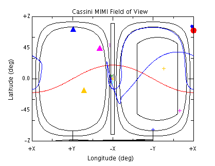
The check boxes here allow the selection of body trajectories to trace in the field of view based plots. See Figure 17, “Titan Trajectory Trace” for an illustration of the trace of Titan. The blue curve represents the path of Titan through the sky.
Unfortunately this feature of JCSN is partially implemented. The traces render only in the spacecraft field of view plot. They also remain on top of the plot as time or orientation are adjusted, but the points along the trace may not be recomputed to reflect the new position or orientation. For now, it is best to consider utilizing this feature only to obtain a snapshot of the trace.
JCSN provides a variety of spacecraft attitude models to supply the application with spacecraft orientation. Only a single model is active at any given moment in a JCSN session. The model is selected by using the combo box at the top of the attitude panel as illustrated in Figure 18, “Selecting the Spacecraft Attitude Model”.
The remainder of this section focuses on discussing the specifics of each attitude model and their individual configurations.
PDT is the Cassini pointing design tool. JCSN supports some of the pointing design rules that PDT provides users for commanding Cassini spacecraft attitude. This section discusses how to use the PDT pointing controls to define spacecraft attitude for the JCSN session.
The supported PDT pointing model defines the spacecraft attitude for the JCSN session by directing vectors in the spacecraft frame to point at specific targets. A primary axis is specified in the spacecraft frame and is aligned with a selected target. Then the secondary axis is specified and aligned as closely as the primary axis lock on its target will permit.
| |
It is possible to specify primary and secondary axes that are in direct conflict with one another, thereby preventing the proper definition of the spacecraft attitude. (For example, pointing Z and Y at the same target for primary and secondary axes). When this happens JCSN will mark the attitude as invalid and cease the display of any quantities dependent on the attitude. There is also the possibility that the primary and secondary targets will end up co-aligned as a consequence of the specific geometry at some epoch. This is frequently a temporary situation that is resolved by nudging the time forward or backward. |
The control interface illustrated in Figure 19, “PDT Pointing Model Interface” is divided into five sections, the primary body axis, the secondary body axis, the primary target, the secondary target, and the supplemental rotation axis controls. The controls presented in each section are discussed in PDT User Controls.
PDT User Controls
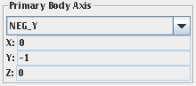
- Body Axis Controls
The interface for controlling the primary and secondary body axes are identical. These controls allow the specification of the body axes which are to be pointed at their respective targets. The combo box at the top of the section presents a list of spacecraft body vectors which are candidates for pointing control. The controls are illustrated in Figure 20, “Body Axis Controls”. For a discussion of the body axes presented in the combo box, see Section 4.1.3, “Pointing Body Axes”.
Selecting a vector from the list causes its immediate assumption of the role of primary or secondary pointing vector. The X, Y, and Z components of the vector in the spacecraft frame are displayed directly underneath the combo box. There are two special exceptions to the general supported body vectors that occur at the end of the list in the combo box.
The first exception, the “RA and DEC” option, changes the controls to allow the specification of the pointing axis in the spacecraft frame by supplying a right ascension and declination. This is illustrated in Figure 21, ““RA and DEC” Controls”.
Angles are specified in degrees. Clicking in the text box and changing the right ascension or declination and then hitting Enter causes the pointing axis definition to change. As with most JCSN text boxes, neglecting to hit Enter results in the display changing but not updating the pointing model.
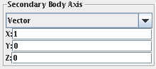
The second and final exception, the “Vector” option, unlocks the vector components to allow the specification of an axis in the spacecraft frame by supplying the three vector components, as shown in Figure 22, ““Vector” Controls”.
To define a pointing axis in the spacecraft frame, click on the text box of the components, edit the contents, and hit Enter to accept the changes. The vector is not required to be a unit vector, but it must not be the zero vector.
- Target Selection Controls
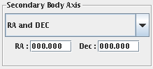
The interface for controlling the primary and secondary target selections are identical. These controls allow the selection of targets at which the corresponding body axes are to be pointed. The combo box at the top of the section presents a list of candidate pointing targets The controls are illustrated in Figure 23, “Target Selection Controls”. For a discussion of the various targets provided in the combo box, see Section 4.1.4, “Pointing Targets”.
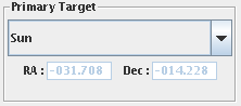
Selecting a target from the list causes the corresponding body axis to immediately be pointed at it. The right ascension and declination in the EME2000 inertial frame are displayed in the text boxes below the target combo box. There are three exceptions to the general target selection interface that occur at the end of the list.
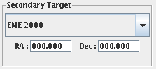
The first exception, “EME 2000”, adjusts the controls to allow the specification of a pointing target in the inertial coordinate frame by supplying a right ascension and declination directly. This is illustrated in Figure 24, ““EME 2000” Target”.
The angles are specified in degrees. Clicking in either text box, changing the angle, and then pressing Enter causes the pointing axis definition to change. Neglecting to hit Enter will result in the displayed angle changing, but the model will not receive the updated value.
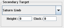
The remaining two exceptions are the “Saturn Limb” and “Titan Limb” targets. These targets provide the same set of controls, but one focuses on Saturn and the other Titan. The Saturn controls are displayed in Figure 25, “Limb Target”.
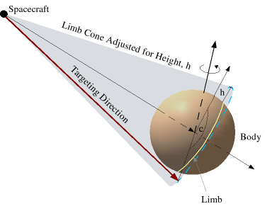
Height is specified in kilometers, and the clock angle is specified in degrees. The targeting direction is selected from the cone with the spacecraft at its vertex and the edges defined by the limb of the spherical model for the body as seen from the spacecraft plus the height adjustment. The clock angle selects the specific vector from the edge of this cone, and is measured off the projection of the body's rotation axis into the plane normal to the cone's axis of symmetry in a right handed sense about the spacecraft-body vector. See Figure 26, “Limb Targeting Geometry” for a diagram of the targeting geometry.
- Supplemental Rotation Controls
The PDT rotation model provides an additional set of controls to define a rotation that sits between the spacecraft frame and the PDT targeting rotation:
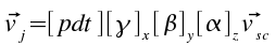
where
The panel illustrated in Figure 27, “Supplemental Attitude Controls” allows the specification of the supplemental rotation angles, in degrees, about each of the spacecraft axes. Clicking the on either side of the angle text box increments or decrements the reported angle. Changing the angle by clicking in the text box and hitting Enter will work as well.
Changing the angle, but neglecting to hit Enter will result in the new angle's display. However, the rotation model will not actually update the rotation matrix until Enter is pressed.

This section lists all of the supported pointing body axes along with a terse description. To view the actual components of the various vectors in the spacecraft frame, refer to the JCSN application PDT pointing GUI itself.
- POSX
The positive X-axis of the spacecraft frame.
- POSY
The positive Y-axis of the spacecraft frame.
- POSZ
The positive Z-axis of the spacecraft frame.
- NEGX
The negative X-axis of the spacecraft frame.
- NEGY
The negative Y-axis of the spacecraft frame.
- NEGZ
The negative Z-axis of the spacecraft frame.
- LGA2
The boresight of LGA-2, one of the low gain antennae on the spacecraft.
- SRUA
The boresight of SRU-A, one of the stellar reference units on the spacecraft.
- SRUB
The boresight of SRU-B, one of the stellar reference units on the spacecraft.
- MEA_PREAIM
Body axis taken directly from PDT. REQUIRES explanation.
- MEB_PREAIM
Body axis taken directly from PDT. REQUIRES explanation.
- CRITICAL_BODY
Body axis taken directly from PDT. REQUIRES explanation.
- XBAND
The boresight of the X-band antenna.
- ISS_NAC
The boresight of the ISS narrow angle camera.
- CIRS_FP1
The boresight of the CIRS focal plane 1.
- CIRS_FP3
The boresight of the CIRS focal plane 3.
- CIRS_FP4
The boresight of the CIRS focal plane 4.
- ISS_WAC
The boresight of the ISS wide angle camera.
- UVIS_HSP
The boresight of the UVIS high speed photometer.
- UVIS_FUV
The boresight of the UVIS far ultraviolet spectrometer.
- UVIS_EUV
The boresight of the UVIS extreme ultraviolet spectrometer.
- VIMS_IR
The boresight of the VIMS infrared channel.
- VIMS_IR_SOL
The boresight of the VIMS infrared channel solar port.
- VIMS_VIS
The boresight of the VIMS visible channel.
- VIMS_RAD
The direct exposure direction of the VIMS radiator.
- RA and DEC
The exceptional body axis that allows the specification of a look direction in the spacecraft frame using right ascension and declination.
- Vector
The exceptional body axis that allows the specification of a look direction in the spacecraft frame by providing the components of the vector directly.
This section lists all of the supported targeting directions along with a terse description of each direction. To view the actual right ascension and declination, refer to the JCSN application PDT pointing GUI itself.
- Sun
The vector connecting the spacecraft to the center of the Sun.
- Saturn
The vector connecting the spacecraft to the center of Saturn.
- Earth
The vector connecting the spacecraft to the center of Earth.
- Mimas
The vector connecting the spacecraft to the center of Saturn's moon Mimas.
- Enceladus
The vector connecting the spacecraft to the center of Saturn's moon Enceladus.
- Tethys
The vector connecting the spacecraft to the center of Saturn's moon Tethys.
- Dione
The vector connecting the spacecraft to the center of Saturn's moon Dione.
- Rhea
The vector connecting the spacecraft to the center of Saturn's moon Rhea.
- Titan
The vector connecting the spacecraft to the center of Saturn's moon Titan.
- Hyperion
The vector connecting the spacecraft to the center of Saturn's moon Hyperion.
- Iapetus
The vector connecting the spacecraft to the center of Saturn's moon Iapetus.
- Saturn Spin Axis
The vector directed along the rotational axis of Saturn.
- Saturn Orbit North
The vector normal to the orbital plane of the Saturnian system directed towards the ecliptic north.
- Saturn Dipole Field
The vector directed along the dipole axis of Saturn's magnetic field.
- Relative Saturn Corotating Plasma
The vector directed along the direction of the relative plasma motion.
- Relative Keplerian Corotating Dust
The vector directed along the direction of the relative dust motion.
- EME 2000
The exceptional case that allows specification of the target direction by specifying a right ascension and declination in the inertial, EME2000 frame.
- Saturn Limb
The exceptional case that allows specification of the target direction relative to the limb of Saturn.
- Titan Limb
The exceptional case that allows specification of the target direction relative to the limb of Titan.
| |
None of the ephemeris based targeting directions are compensated for light time. |
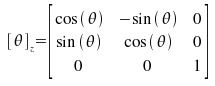
The Euler rotation model allows the specification of spacecraft attitude relative to the inertial reference frame (EME2000) by utilizing Euler angles. Figure 28, “Euler Rotation Model Interface” illustrates the user interface controls.
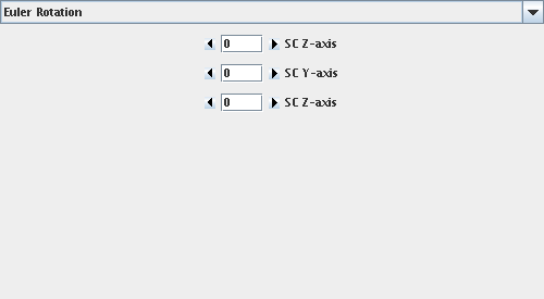
The angles are specified in degrees. The rotations about the three axes are applied in a top to bottom fashion to vectors in the spacecraft frame to produce vectors in the inertial frame (EME2000). Clicking the on either side of the angle text box increments or decrements the reported angle. Changing the angle by clicking in the text box and pressing Enter will work as well. See Figure 29, “Euler Angle Configuration” for a detailed diagram of the combination of these three rotations.
| |
Changing the angle, but neglecting to hit Enter will result in the new angle's display. However, the rotation model will not actually update the rotation matrix until Enter is pressed. |
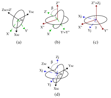
(a), (b), and (c) illustrate the application of the Euler angles to rotate vectors from the spaecraft to inertial frame. (d) illustrates the composition of the entire Euler angle sequence.
Figure 29. Euler Angle Configuration
| |
The definition of Euler angles that JCSN utilizes results in a series of “left-handed” rotations about the principal axes. This is contradictory to the typical definition of such angles, though it is really just a matter of perspective. |
The first rotation about the Z-axis specified at the top of the interface panel is applied in (a). The black vectors represent the spacecraft axes. The green, primed, vectors are the result of application of the first Euler angle. In (b), the green vectors continue to represent the spacecraft axes after the application of the first Euler angle. The red, double-primed, vectors are the frame axes after the application of the second rotation about the Y-axis. The final Euler rotation is presented in (c). The red vectors represent the composition of the first two rotations. The blue vectors are the result of the application of the third angle, and are the axes of the inertial frame. (d) illustrates the combination of the three rotations and the angles as a result.
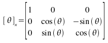
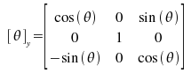
For reference, the rotation matrix from the spacecraft to inertial frame is computed:
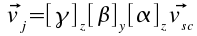
where:
and
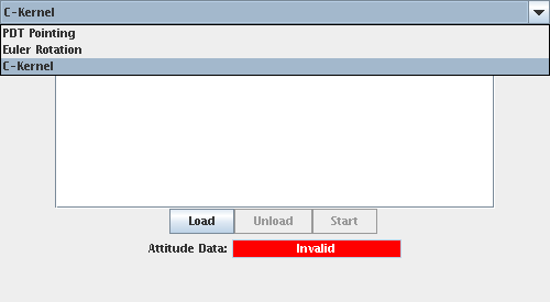
The C-kernel rotation model reads JPL's SPICE instrument and spacecraft pointing data files, or simply C-kernels, to determine orientation. This section discusses the details of how to properly utilize these files to provide spacecraft attitude, and how JCSN handles any data “drop-outs” that can and do occur.
As Figure 30, “C-kernel Model Interface” illustrates, when the C-kernel model is first selected the list of loaded kernels is empty.
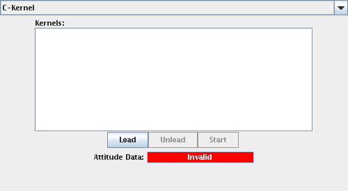
The interface consists of three distinct parts: the loaded kernel list, the control buttons, and the attitude validity indicator. Each of these are discussed in C-kernel User Controls.
C-kernel User Controls
- Loaded Kernel List
This element of the interface lists all C-kernels currently loaded into JCSN. The order is significant, as the kernels at the top of the list have the lowest priority when locating attitude for the spacecraft.
- Control Buttons
These buttons allow loading and unloading of kernels, as well as browsing to the start of a particular kernel.
- Indicator
This light indicates whether the C-kernel model is providing data for the plot panels rendered belown and time functions displayed to the left. If the light is red, the scenes are generated using attitude from the last successful attitude computation.
This may or may not be representative of the actual spacecraft attitude at the displayed time.
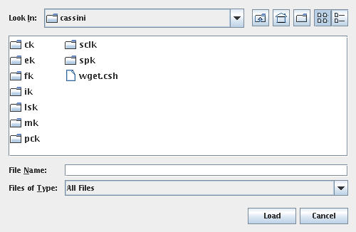
Loading a C-kernel into JCSN is as simple as clicking the load button. A dialog box, as illustrated in Figure 31, “The “Load C-kernel” Dialog” will appear. Select any Sun binary formatted C-kernel available on your system and click . See Section 4.3.5, “Cassini C-kernel Naming Conventions” for details on the file naming conventions.
| |
If something goes wrong when JCSN is attempting to load the C-kernel a dialog box indicating a failure, such as the one show in Figure 32, “The “Unable to Load C-kernel” Dialog” will appear. |
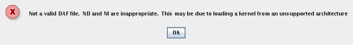
A properly formatted and constructed C-kernel can fail to load for two reasons:
The C-kernel is not in “big endian” format. The SPICE toolkit is capable of reading C-kernels presented in both big and little endian formats. The current release of JCSN reads only kernels delivered in big endian format. Fortunately all of the C-kernels delivered by Cassini AACS are in this format.
Due to the way the kernels are read into the application, they are loaded into memory in their entirety. If the virtual machine runs out of memory, you will be unable to load additional C-kernels. Unload one or more of the loaded kernels to make room for the new one.
Once the C-kernel is loaded into JCSN, it will appear in the “Kernels:” list as show in Figure 33, “The Button”.
When a kernel is loaded and selected in the “Kernels:” list, the and buttons are enabled. Clicking removes the currently selected kernel from the applications resource pool. Clicking on the button sets the state of JCSN to the reported start of the selected kernel, as shown in Figure 33, “The Button”.
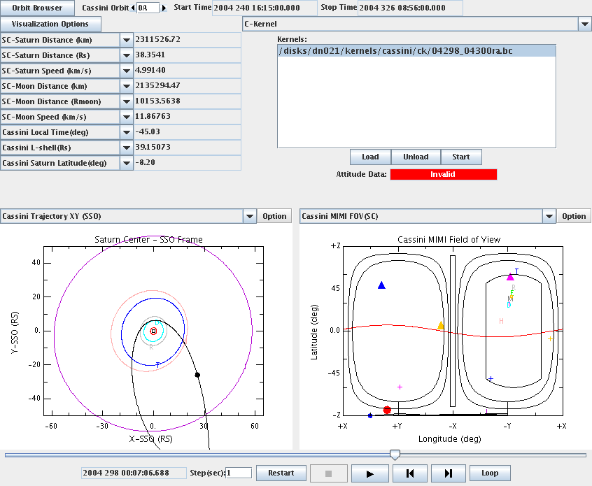
| |
Occassionally, as illustrated in Figure 33, “The Button”, after selecting a loaded kernel and clicking , the attitude validity indicator remains set to “Invalid”. This happens because of the way JCSN rounds the displayed time. Simply taking a small step forward in time of a second or so, should result in the validity indicator changing to “Valid”. |
After loading the set of kernels that cover the period of in which you are interested, select the desired two plot panels and time functions. Then you can use JCSN just as you would with the PDT Pointing or Euler Angle Rotation models. As long as the Attitude Data: is white and reports “Valid”, the data used to present the display is derived directly from the C-kernel. If it turns red and displays “Invalid”, then the attitude used to generate the display is the previously computed attitude. This may or may not be appropriate.
So the next question is at this point: how does one fill the gaps in reconstructed C-kernels with something meaningful? The project recommends supplementing reconstructed attitude data with predict data. Take for example the reconstruction near the first Titan flyby illustrated in Figure 34, “Reconstructed Attitude Dropout”.
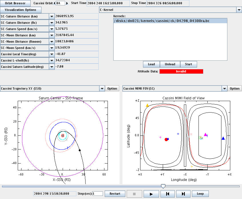
Since JCSN takes attitude data from the C-kernels loaded last as the highest priority, load the corresponding predict data first. Then load the reconstructed data and JCSN will automatically fill any gaps in the attitude telemetry with the predict data. For example, see Figure 35, “Reconstructed Data Supplemented with Predict”
Observe, now that the predict data is available, the Attitude Data: is reporting “Valid” where it was reporting, in Figure 34, “Reconstructed Attitude Dropout”, “Invalid”.
| |
Loading predict C-kernels that cover the period of interest after loading the reconstructed C-kernels will result in JCSN only providing access to the predict data. The reconstructed data will effectively be masked by the predict. |
The official Cassini project SPICE kernel archive is located
at ftp:kernels/ck directory underneath this URL.
There is a local copy of the C-kernel repository kept at APL
at http:
NAIF maintains the official document describing the Cassini
C-kernel conventions at:
ftp:
           [StartDate]_[EndDate][Type][V]_[xxxxxxxx].[Ext]

   where:

              [StartDate]   File coverage start date (YYDOY);

              [EndDate]     File coverage stop date (YYDOY);

              [Type]        Type of the data stored in the file: ``r'' =
                            reconstruction, ``p'' = predict;

              [V]           File version. The first file generated for a
                            specific time frame is version ``a''. Subsequent
                            files containing revised information for the same
                            time period are given the next higher version
                            letter -- ``b'', ``c'', etc;

              [xxxxxxxxx]   Optional freeform text that describes the sequence
                            phase for which the file was created.

              [Ext]         Standard SPICE extension for CK files: ``bc'' for
                            IEEE binary CK files, ``xc'' or ``tc'' for
                            transfer format CK files.

   For example, the file:

           03215_03220pa_port1.bc

   is a binary CK containing predicted data and covers a time period in 2003
   from day of the year 215 to 220. It is the first version created for the
   port 1 sequence generation.
Prior to this date, the “StartDate” and “EndDate” were populated with the YYMMDD format, instead of day of year.
If two kernels have precisely the same name, but differ only in the “Version” field, always load the latest offered revision.
| |
If the kernel you are interested in loading into JCSN has the extension “.xc” rather than “.bc”, then this file is presented in SPICE transfer format. There are tools distributed with the SPICE toolkit for converting transfer format kernels to binary format. See the toolkit installation documents for details. |
The C-kernel attitude history rotation model reads a set of JPL's SPICE C-kernels that are produced locally at APL. These files are merged and lossy compressed to a tolerance of 1 milliradian. The resultant kernels are supplied at load time to JCSN to be utilized by this attitude model. It attempts to provide spacecraft attitude coverage for the entire tour.
Using this model is as simple as selecting it from the drop down box, and just examining the data in JCSN. There are two separate attitude sources that are loaded into the application: a predict and a reconstructed set. The reconstructed set is compressed spacecraft attitude history telemetry. The predict set is compressed attitude predicts produced during the mission planning and sequencing process. The predict data is used by JCSN only to gap fill the reconstructed data.
The only display on the interface is a source indicator, which illustrates the source of the attitude used to render the currently selected time in JCSN. The following figures illustrate the three possible states the indicator assumes and their respective meanings.
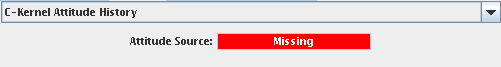
Illustrates the attitude source indicator's state when the spacecraft attitude is missing from both sources at the currently rendered time.
Figure 36. C-kernel Attitude History Missing Source Data
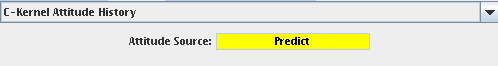
Illustrates the attitude source indicator's state when the spacecraft attitude is only available from the predict source.
Figure 37. C-kernel Attitude History Predict Only Source Data
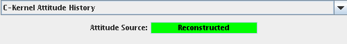
Illustrates the attitude source indicator's state when the spacecraft attitude is only available from the predict source.
Figure 38. C-kernel Attitude History Reconstructed Source Data
| |
When the attitude source indicates the “Missing” state, there is no spacecraft attitude data to render the plots and time functions. JCSN simply uses the last value it cached from a time when data was available. |
The JCSN time functions display a variety of geometric quantities that are evaluated at the current epoch the application is rendering. These functions include longitude, latitude, speeds, distances, as well as right ascensions and declinations of the spacecraft axes.
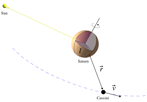
The vectors r and v illustrate the position and velocity of Cassini relative to Saturn. The angle l measures local time in degrees from noon.
Figure 39. Sun, Saturn, and Cassini
Figure 39, “Sun, Saturn, and Cassini” Time Functions
- SC-Saturn Distance (km)
The magnitude of the vector r expressed in kilometers. This is the distance between Cassini and Saturn's body center.
- SC-Saturn Distance (Rs)
The magnitude of the vector r expressed in Saturn body radii. This is the distance between Cassini and Saturn's body center.
- SC-Saturn Speed (km/s)
The magnitude of the vector v expressed in kilometers/second. This is the speed of Cassini's motion relative to Saturn's body center.
- Cassini Local Time (deg)
The angle l expressed in degrees from local noon. This is the Saturnian local time of Cassini's position.
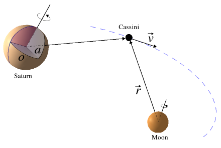
The vectors r and v illustrate the position and velocity of Cassini relative to the displayed Moon. The angles a and o measure the latitude and longitude of Cassini respectively. The blue line of longitude on Saturn marks the prime meridian, from which o is measured.
Figure 40. Saturn, Reference Moon, and Cassini
Figure 40, “Saturn, Reference Moon, and Cassini” Time Functions
- SC-Moon Distance (km)
The magnitude of the vector r expressed in kilometers. This is the distance between Cassini and the selected reference moon's body center.
- SC-Saturn Distance (Rmoon)
The magnitude of the vector r expressed in the selected reference moon body radii. This is the distance between Cassini and the moon's body center.
- SC-Moon Speed (km/s)
The magnitude of the vector v expressed in kilometers/second. This is the speed of Cassini's motion relative to the selected reference moon's body center.
- Cassini Saturn Latitude (deg)
Angle a measures the latitude on Saturn of Cassini's position. This time function displays the value of the latitude measured in degrees.
- Cassini Saturn Longitude (deg)
Angle o measures the longitude on Saturn of Cassini's position. This time function displays the value of the longitude measured in degrees from the prime meridian.
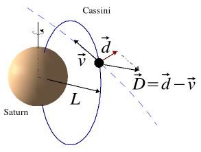
The vectors d and v are the dust and Cassini velocities relative to Saturn respectively. The blue curve marks a simple dipole magnetic field line on which Cassini is sitting. The length of vector L is the L-shell. The vector D is the velocity of the dust as observed from Cassini.
Figure 41. Saturn and Cassini
Figure 41, “Saturn and Cassini” Time Functions
- Cassini L-shell (Rs)
The length of vector L expressed in units of Saturnian radii. This is the dipole L-shell of Cassini's position.
- Dust relative velocity (km/s)
The length of vector D, the speed of the dust motion as observed from Cassini's position. This vector is the result of subtracting Cassini's velocity from the dust velocity. The length is expressed in kilometers/second.
Other Available Time Functions
- +X - Sun Angle (deg)
The angle expressed in degrees between the spacecraft +X axis and the Sun.
- +X Axis RA (deg)
The right ascension of Cassini's +X axis expressed in degrees.
- +X Axis Dec (deg)
The declination of Cassini's +X axis expressed in degrees.
- +Y Axis RA (deg)
The right ascension of Cassini's +Y axis expressed in degrees.
- +Y Axis Dec (deg)
The declination of Cassini's +Y axis expressed in degrees.
- +Z Axis RA (deg)
The right ascension of Cassini's +Z axis expressed in degrees.
- +Z Axis Dec (deg)
The declination of Cassini's +Z axis expressed in degrees.
- -X Axis RA (deg)
The right ascension of Cassini's -X axis expressed in degrees.
- -X Axis Dec (deg)
The declination of Cassini's -X axis expressed in degrees.
- -Y Axis RA (deg)
The right ascension of Cassini's -Y axis expressed in degrees.
- -Y Axis Dec (deg)
The declination of Cassini's -Y axis expressed in degrees.
- -Z Axis RA (deg)
The right ascension of Cassini's -Z axis expressed in degrees.
- -Z Axis Dec (deg)
The declination of Cassini's -Z axis expressed in degrees.
JCSN provides a variety of plots to display data to the users.
This section is a placeholder until the actual section content is complete.
JCSN displays data computed in a variety of coordinate systems. This section defines the systems in use throughout the application and this documentation.
There are several types of reference frames and coordinate systems used in JCSN. Reference Frame Classifications enumerates them with a brief description.
Reference Frame Classifications
- Inertial
The axes of these frames are fixed and do not rotate with respect to the orbital motion of the planets or the background star field. Thus, Newton's laws of motion apply in frames of this class.
- Body-Fixed
The axes of these frames are tied to a particular body, often defined relative to its features in some fashion. As such, the axes rotate rigidly with the body. The spacecraft frame and the IAU body-fixed reference frames are simple examples of these types of frames.
- Dynamically Defined
These frames are defined by selecting axes from various orbital geometry vectors that may evolve in time. Typically a primary vector is selected and labeled. Then a secondary vector is chosen, which another labeled axis points as close as it can to, given the constraint of the primary pointing vector. The third and final axis is the result of completing the right-handed frame definition.
The EME2000 frame is the inertial reference frame against which all ephemerides and frame transformations in JCSN are computed. The definition of EME2000 JCSN utilizes is consistent with the standard IAU definition.
The spacecraft frame is the reference frame tied to the Cassini orbiter body. CHEMS's look direction is parallel to the -X axis in this frame, while INCA's is parallel to a vector rotated 9.5 degrees off the -Y axis.
All celestial body-fixed reference frames in JCSN are defined in a manner consistent with the IAU standards. The Z-axis of these frames is directed parallel to the rotation axis of the body. The X-axis marks the intersection of the prime meridian and the body's equator. The Y-axis completes the right-handed frame.
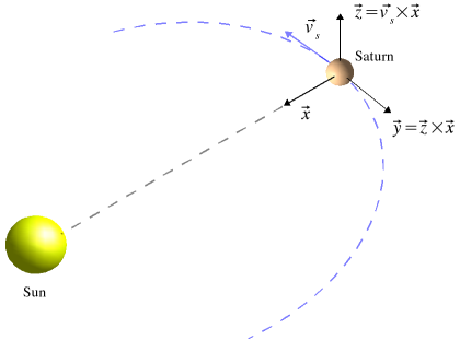
The Saturn Solar Orbit (SSO) frame is a dynamically defined frame. As illustrated in Figure 42, “Saturn Solar Orbit (SSO) Configuration”, the primary axis is a vector parallel to the Saturn-Sun line and is labeled X. The Z-axis is the result of the cross product of Saturn's velocity vector relative to the Sun with the primary axis. The Y-axis completes the right-handed system.
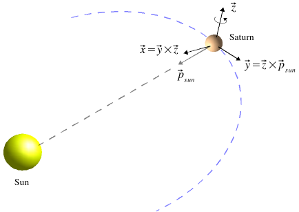
The Saturn Equatorial System (SZS) frame is another dynamically defined frame whose axes are selected from various orbital geometry vectors. Figure 43, “Saturn Equatorial System (SZS) Configuration” demonstrates the selection of the vectors. The primary axis, labeled Z, is parallel to the Saturn spin axis. The Y-axis is then defined as the cross product of this vector with the Saturn-Sun vector. The X-axis completes the right-handed system and is directed “towards” the Sun.
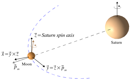
Another dynamically defined frame, the Corotation frame has as its primary axis the Saturn spin axis, labeled Z. The Y-axis is then defined to be the result of crossing this vector with the Saturn-ReferenceMoon vector. The X-axis completes the right-handed frame definition and is directed away from Saturn as illustrated in Figure 44, “Corotation Configuration”.
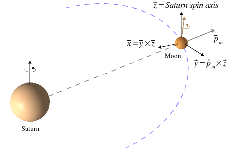
The Saturn Moon System (SZM) frame is a dynamically defined frame whose primary axis, labeled Z, is the Saturn spin axis. The Y-axis of this frame is chosen to be the cross product of the Saturn-ReferenceMoon vector and this Z-axis. The X-axis completes the right-handed frame. The Saturn Moon System (SZM) frame is almost exactly the same as the Corotation frame, but its X and Y axes point in opposite directions.
JCSN utilizes several models and makes some assumptions to compute or present the displays. This section summarizes these briefly.
The magnetic field is a simple dipole aligned with the Saturn spin axis with no offset.
The dust model is a simple cylindrical [1] Keplerian model.
The plasma model is a cylindrical [1] corotation model.
All ephemeris objects are computed as geometric states with no light time or stellar aberration corrections applied to them.
Time is specified in ephemeris time, or Barycentric Dynamical Time (TDB).
Position and velocities are obtained from SPICE kernels.
Planet and moon rotation models are the standard IAU body rotation models.
[1] Cylindrical is inserted to imply that particles with the same cylindrical coordinate radius have precisely the same velocity.