Analysis software is available on line for INCA. The applications include
PHA plots which are shown above, pitch angle versus flux plots, TOF spectrograms, and
TOF channel plots, which are also shown above. The image skymaps can be viewed in
a single image format which is shown in the movie description, and the multiple format is
shown in both the ENA and ION image calibrated products.
NOTE: Currently the IDL tools will only work
with version 3 and higher of the MIMI PDS Data. The version 3 files are available 2007-2011. Years
2004-2006 will be coming soon.
Goto Descriptions
|
Goto Applications
|
|
|
|
|
|
Time Menu Description
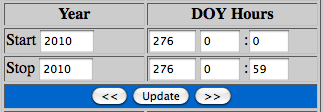 Start and stop time format is yyyy-doyThh:mm.
Year is a 4 digit year. DOY is the day-of-year which goes from 1
to 365 on non-leap years and 366 on leap years.
The hh is the 2 digit hour and mm is the 2 digit
minutes fields respectively. Valid values for hours is 0-23 and valid values for minutes is 0-59. On some menus due to the window width, the minute fields may display
below the hours.
To page from one day to the next, use the << or >> buttons.
To page across more than one day, edit the Amount (doys) field and use the << or >> buttons. |
|
|
|
|
INCA PHA Plot DescriptionGoto INCA PHA Plot
| Example | 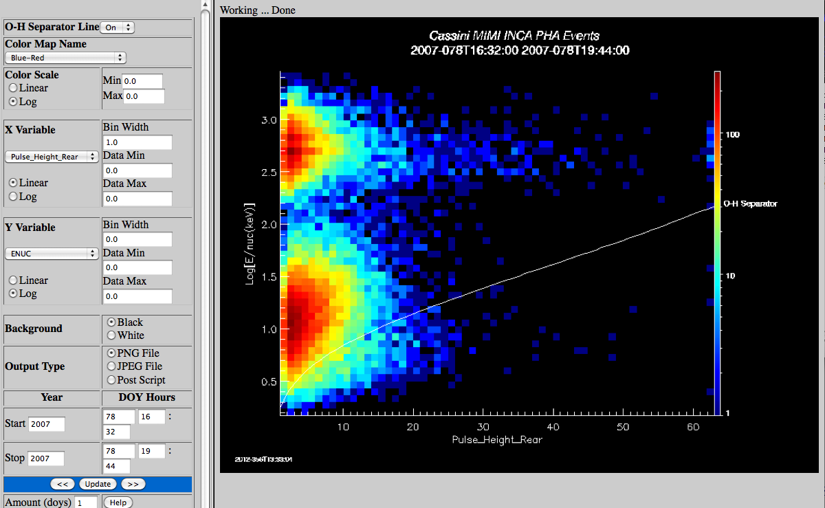 |
| OH separator line | Select the whether to plot the Oxygen-Hydrogen separator line. It can only be plotted when
Pulse_Height_Rear is being plotted versus ENUC. |
| Color Map Name | List of IDL colormap names, default is Blue-red. |
| Colorscale | The colorscale can be calculated as linear or log. The minimum and
maximum value are always entered as linear numbers. Set the values to 0.0 and let the software default to the images maximum and minimum. |
| X Variable |
Coinc - This field identifies whether the PHA event includes a coincidence.
Start/Stop - This field identifies whether the PHA event included both start and stop(1) or only one of the
two (0).
Pulse_height_front - This field contains the encoded pulse height data for the front (Start) microchannel
plate. It was added on 2000-154 and is not present before that date.
Pulse_height_rear - This field contains the encoded pulse height data for the rear (Stop) microchannel
plate. It was added on 2000-154 and is not present before that date. This is the default value for X
variable.
TOF - This field contains the PHA event 10 most significant bits of the on-board-corrected particle time of
flight in data numbers.
ENUC - This field is energy per nucleon and is calculated from the TOF and the units are
E/num(kev). This is the default value for the Y variable.
Azimuth - This field contains the encoded value of the calculated azimuth for the PHA event. Azimuth ranges
are from 0 to 63 (-90 to 90 degrees).
Elevation - This field contains the encoded value of the calculated elevation for the PHA event. Elevation
ranges are from 0 to 47. (-60 to 60 degrees).
Mass Range - This field contains the encoded value of the calculated mass.
The X variable can be plotted as linear or log. The default value of
the bin width is 1.0. The default data minimum and maximum are 0.0 which will make the software
plot using the data minimum and maximum. |
| Y Variable | The Y variables are the same as the X variables and the default value is ENUC. The ENUC variable is a value
calculated from the TOF. The X variable can be plotted as linear or log. The default value of
the Y bin width is 0.0. The default data minimum and maximum are 0.0 which will make the software
figure out the data minimum and maximum. |
| Background | The plot background can be black or white |
| Ouput Type | The user can select to plot PNG, JPEG or post script output files. For the File output types click on the File label with the right mouse button and use Save Link Target. |
|
|
|
|
|
INCA Pitch Versus Flux Plot DescriptionGoto INCA Pitch Versus Flux Plot
Scatter
Plot
Example | 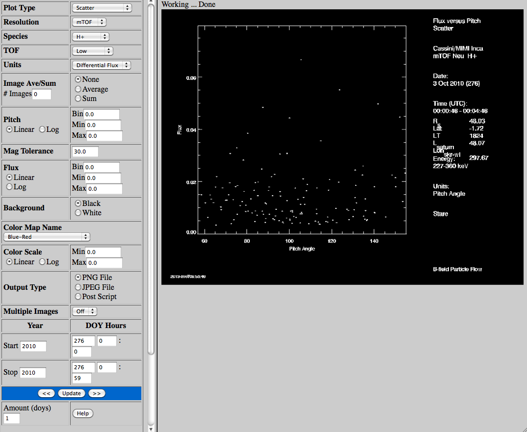 |
Color
Histogram
Example | 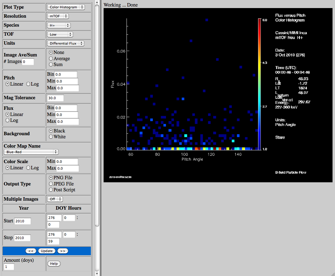 |
| Plot Type | Select the plot type, either a scatter or color histogram of INCA pitch angle on the X
axis and image flux on the Y axis for one image. |
| Image Type | Select the Image Resolution, Species and TOF.
High Spatial images can be species Hydrogen or Oxygen and can be Low or High TOF.
High Time images do not differentiate between species so either value will work. Select from low or high TOF.
High mTOF images can be species Hydrogen or Oxygen and can be Low or High TOF. |
| Units | Select the units, the tof channel data can be displayed in counts, integral flux or differential flux. |
| Ave/Sum | Select Averaging or Summing and the number of images to average or sum. This is good to do when viewing
multiple days data. Averge or sum must be 2 or greater and either Average or Sum must be turned on. |
| Linear/Log | The X (pitch) axis or Y (Flux) axis can be plotted as linear or log. Let the bin width for the pitch angle or flux
be set using the data maximum and minimum (max-min)/50 or input a width. |
| Minimum/Maximum | Let the pitch angle or flux data maximum or minimum be set using the data or select a range. These are in the range of the
variable type. |
| Color Map Name | List of IDL colormap names, default is Blue-red. |
| Mag Tolerance | The magnetometer tolerance value will prevent plotting the data if the mean of the
magnetometer data is greater. |
| Background | The plot background can be black or white |
| Ouput Type | The user can select to plot PNG, JPEG or post script output files. For the File output types click on the File label with the right mouse button and use Save Link Target. |
| Multiple Images | Each plot contains data from only one image. To plot data from multiple images, turn on
this flag. Beware, if you select too much data (especially when using high time resolution images), it may take a while to plot all the data. Also, use average or sum to average
or sum the data from multiple images into one plot. |
|
|
|
|
|
INCA TOF Spectrograms Plot DescriptionGoto INCA TOF Spectrograms
| Example | 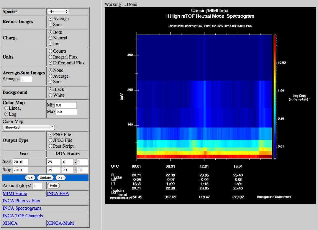 |
| Species | Select the Image Species. High mTOF images can be species Hydrogen or Oxygen. |
| Reduce Images | Select the Reduce Images option, either average or sum all pixels in an image to a single point. |
| Charge | Select the Image Charge Mode, both modes, or only Neutral or Ion mode data. |
| Units | Select the units from counts, integral flux or differential flux. |
| Average/Sum | Select Averaging or Summing and the number of images to do. This is good when viewing multiple days
data, usually more than one week. |
| Color Map Name | List of IDL colormap names, default is Blue-red. |
| Background | The plot background can be black or white |
| Select the color map option. |
| Colormap Min/Max | Enter a minimum and maximum range for the color map or let the software default to the images maximum and minimum. |
| Background | The plot background can be black or white |
| Ouput Type | The user can select to plot PNG, JPEG or post script output files. For the File output types click on the File label with the right mouse button and use Save Link Target. |
|
|
|
|
|
INCA TOF Channel Plot DescriptionGoto INCA TOF Channel Plot
| Example | 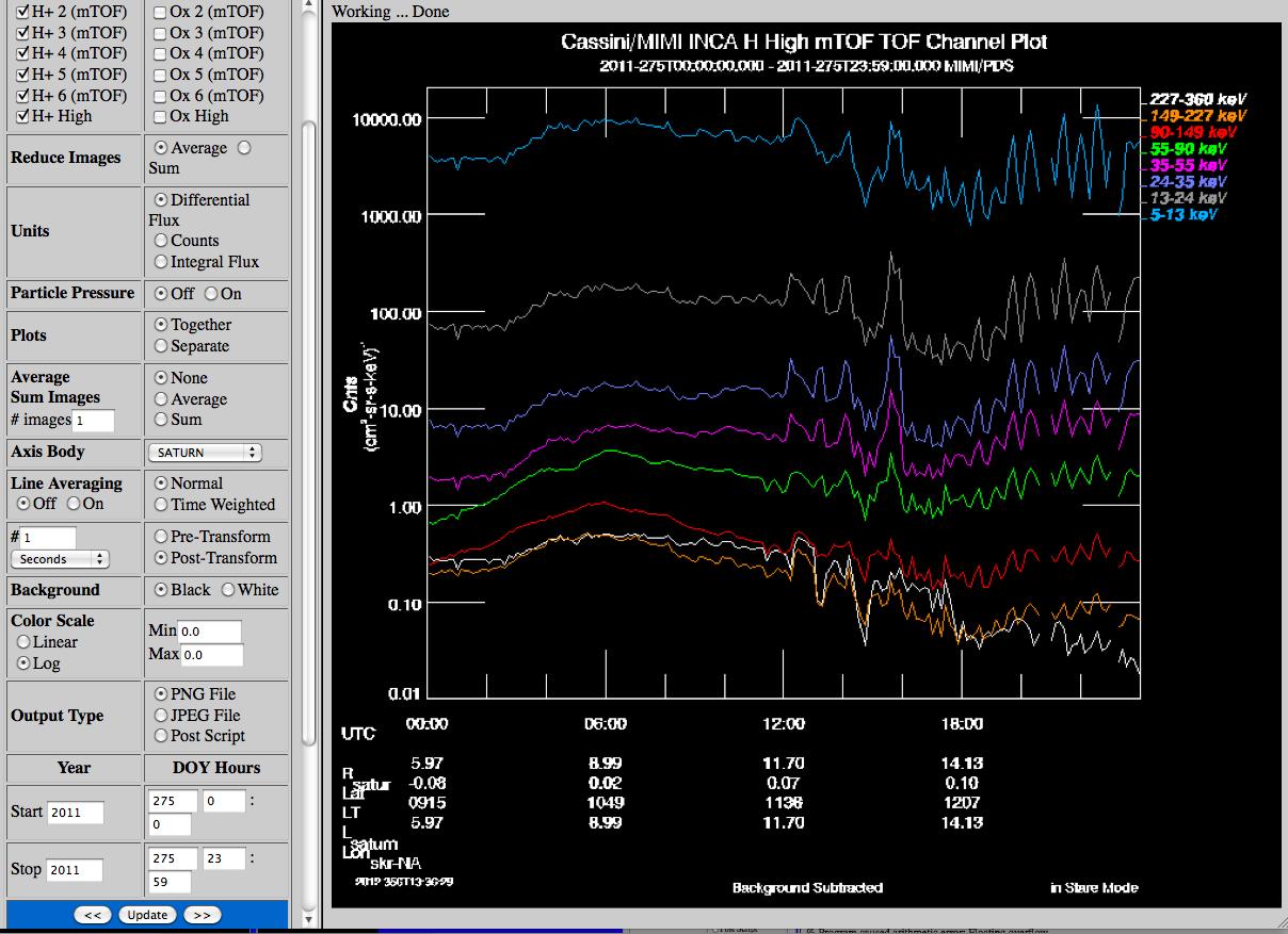 |
| Resolution | Select the Image Resolution type.
|
Species
TOF | Select the Image Species and TOF.
High Spatial images can be species Hydrogen or Oxygen and low or high TOF.
High Time images does not differentiate species but does have either low or high TOF
High mTOF images can be species Hydrogen or Oxygen and low, 1, 2, 3, 4, 5, 6 or high TOF. |
| Reduce Images | Select the Reduce Images option, either average or sum all pixels in an image to a single point. Average is the default for
flux. |
| Charge | Select the Image Charge Mode, both modes, or only Neutral or Ion mode data. |
| Units | Select the units from counts, integral flux or differential flux. |
| Particle Pressure | This option changes works with the following parameter plots to change the plot into inca particle
pressure either in individual TOF's or together as one line depending on the value of the plots parameter. |
| Plots | This works with the particle pressure field. Selects to plot the individual TOF together or separately. |
| Average/Sum Images | Select Averaging or Summing and the number of images to do. This is good when viewing multiple days
data, usually more than one week. |
| Axis Body | Select the Axis body for the supplementary labels (radius, latitude, local time) on the time axis. These do not appear
for every plot. The L value will still be for Saturn. |
| Line Averaging | Select if you want to average the data after the pixels have been averaged into a single value.
The normal method of averaging sums the data
over the time range and divides by the number of samples per time range.
The time weighted method of averaging sums the data times it's accumulation time over the
time range and divides by the total accumulation time.
The interval fields allow the user to select a number and interval type: seconds, subsectors, sectors and spins.
The Pre-Transform averaging is better to use for very long time ranges because it reads
the data in one day at a time, averages it and concatenates the data together beform doing any
selected transformations on it.
The Post-Tranform is the default method to use for averaging. It performs the averaging
after any selected transforms have been done. |
| Color Map Name | List of IDL colormap names, default is Blue-red. |
| Background | The plot background can be black or white |
| Select the color map option. |
| Colormap Min/Max | Enter a minimum and maximum range for the color map or let the software default to the images maximum and minimum. |
| Background | The plot background can be black or white |
| Ouput Type | The user can select to plot PNG, JPEG or post script output files. For the File output types click on the File label with the right mouse button and use Save Link Target. |
|
|
|
|
|
INCA Image Skymap DescriptionGoto INCA Image Skymap Plot
| Example | 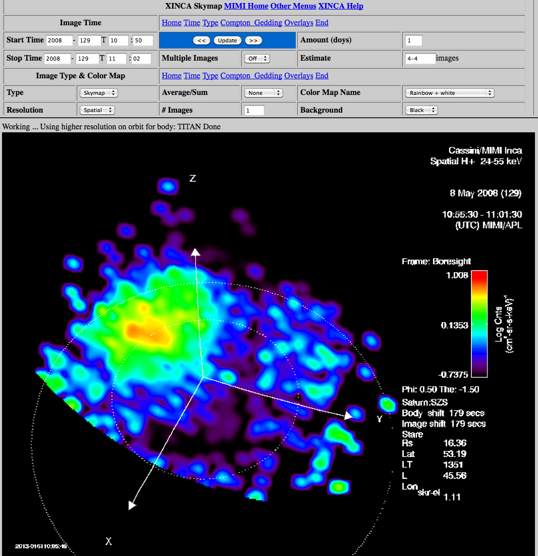 |
Displaying INCA Energetic Neutral Atom (ENA) Images:
The Skymap is the input image projected onto the sphere
of the sky, using the azimuthal projection with the 'north pole' of the sky sphere being the vertical axis.
This display is designed for the analysis of ENA images, produced when the INCA high voltage ion and electron
rejection plates are powered. This display is typically Saturn or Titan centered, in which case the vertical
axis is aligned parallel with the body north pole. Other frames keep the vertical axis in the projected image
parallel with the spacecraft Z axis. Various objects may be chosen for wire - frame overlay representation in
the image display.
Displaying INCA data in Ion Mode: This menu also produces a (selectable) display known as Thumbnail, for with
the INCA FOV is represented in instrument, rectangular coordinates (vertical is elevation, parallel with the
INCA slit and collimator plates, and with the Spacecraft Z axis, horizontal is azimuth, perpendicular to the
INCA slit and collimator plates). This display is the appropriate choice for displaying INCA ion measurements
when the charged particle rejection plates are turned off. Using the on - board magnetic field vector (provided
courtesy of the Cassini MAG Investigation) the contours of constant pitch angle may be used as overlays in the
Thumbnail projections. When the spacecraft is rolling about its Z axis, the coordinates of the Thumbnail map
are the spin based coordinates to represent what a spinning imager 'sees'.
Menu section names are on the left and the links next to them jump to the menu sections. |
Start and Stop
Times | Enter the start and stop year, day of year and hours.
Image Time - DO NOT SELECT A LONG INTERVAL (e.g., days) or the website will stall!
The closest image(s) in time to the selected time will be displayed.
Select "Multiple Pages: Off" to plot only the first image in the set (especially useful when initially
choosing plot parameters) or "On" to plot all the images in the set. (Only the first 20 images will be
plotted, the rest will appear as output file hyperlinks at the top of the window.).
The estimated number of images that will be created is displayed to the right of the time when selected.
This information is intended to help you decide if you have picked too much data for the application to
display. If you select to display more than 25 images, a warning window will appear. Please consider selecting
less than 25 images or do the images in sets since too many will overwhelm the web
server. |
| Update | Select Update Window button.
Click UPDATE to generate output images (but set all other parameters below first!)
To page from one day to the next, use the << or >> buttons.
To page across more than one day, edit the Amount (doys) field and use the << or >> buttons. |
| Select the Image Resolution. |
Spatial produces Hydrogen - - H+ low, H+ high, (where low and high refer to TOF - therefore "low" is higher in
energy than "high". For Spatial H, "low" corresponds to 55keV to 90keV, "high" corresponds to 24keV to 55keV)
or Oxygen - Ox low (170keV - 230keV), Ox high (90keV - 170 keV). The H+ high and both Ox images are at 32 x 32
pixel resolution over the 90 (azimuth) by 120 (elevation) INCA FOV. The H+ low are at 64 x 64 pixel
resolution.
High Time Res. images do not discriminate between species, but are typically dominated by hydrogen. These
images are at 32 x 32 pixel resolution over the 90 (azimuth) by 120 (elevation) INCA FOV. They are produced at
4 times higher cadence than the Spatial and mTOF images.
High mTOF Res. Images, 16 x 16 pixels covering the INCA FOV, are produced for both Hydrogen and Oxygen. They
are each available at 8 energies for each species - for H, they are produced at 5 - 13keV (TOF7 or "high"),
13 - 24keV (TOF6), 24 - 35keV (TOF5), 35 - 55keV (TOF4), 55 - 90keV (TOF3), 90 - 149keV (TOF2), 149 - 227keV (TOF1), and
227 - 360keV (TOF0 or "low"). For oxygen the energies are 46 - 68keV, 68 - 90keV, 90 - 129keV, 129 - 168keV,
168 - 231keV, 231 - 332keV, 332 - 589keV, and 589 - 1000keV. |
| Select the Image TOF and Species. |
High mTOF resolution images have low - high (8 values)
High spatial and time resolution images have only low and high TOF.
|
| Units | Select the units: counts, integral flux or differential flux. |
| Radius,Lat,LT | Select the celestial body relative to which the spacecraft location coordinate values radius, latitude,
local time, L value and SKR Longitude is calculated. |
| Frame | FRAME The desired frame in which sc_pos, spin_axis, and boresight vector are going to be returned in.
Can take the values:
Boresight - The primary (X) axis is the CASSINI_MIMI_INCA boresight axis and is labeled X. The secondary
(Z) axis is the Z axis of the IAU_SATURN frame (Saturn north spin axis vector). The Y-axis completes the
right - handed system.
Saturn - This frame is a dynamically defined frame, defined as follows: the primary axis is the CASSINI
spacecraft - to - Saturn vector and is labeled X. The secondary Z axis is the Z axis of the IAU_SATURN frame.
The Y-axis completes the right - handed system.
Titan - This frame is a dynamically defined frame, defined as follows: the primary axis is the CASSINI
spacecraft - to - Titan vector and is labeled X. The secondary Z axis is the Z axis of the IAU_TITAN frame.
The Y-axis completes the right - handed system.
Saturn SZS - The primary axis, labeled Z, is parallel to the Saturn spin axis. The Y-axis is defined as
the cross product of this vector with the Saturn - Sun vector. The X-axis completes the right - handed system
and is directed "towards" the Sun.
SKR - Projected - This frame is a Saturn centered frame, similar to XINCA_SATURN_CENTERED, as the primary
axis is defined as the spacecraft - Saturn vector. However, instead of utilizing the Saturn - sun vector as
the definition of the proper clock angle about the primary axis, this frame uses the SKR prime meridian.
By SKR, we refer to the currently available source for this information (SLS3, SLS4 south, etc.).
|
Average/Sum
#Images
Width | Select the number of images to sum or average (2 - >) and select the averaging or summing option. The
default is 1, which means no summing or averaging.
Select the width (STEP) between the output averaged or summed images. The Default, 0, has the effect of stepping
forward in time by the number of images chosen for the sum or average, so that each output image is
independent and contiguous. Choosing values other than 0 forces that value to be used. For example, if
you are averaging over 10 images, leaving STEP at 0 means each successive group of 10 input images will be
averaged into a successive output image. Choosing 10 will have exactly the same effect. However,
choosing 1 will result in a "sliding boxcar" average, where 10 input images are averaged to form 1 output
image, then the program moves forward by 1 image accumulation time and forms another 10 image average for
the next output image. This second average will include nine of the images included in the first average,
plus one additional image forward in time. This achieves a sort of morphed sequence of images with strong
persistence from one image to the next in the sequence, suitable for creating movie image frames. |
| Colormap Min/Max | SCALE: Select values by which to scale the images. Leaving the scaling at zero forces automatic color
bar scaling for the images (middle of the menu), by species and TOF (which means each horizontal row (time
axis) in the output matrix of images will be scaled to the same min and max; scale all together (meaning
all of the images in the output matrix will be scaled to the same color bar) or scale them individually
(meaning each output matrix image will be individually scaled to the min/max of the color bar). |
| Smooth | Smooth - Applies a boxcar smoothing function to the mapped image. The purpose is to smooth the visible
image to aid the eye in interpreting the image as a 3D structure and not make the eye unconsciously map it
to the sphere. CAUTION!!: Localized features broaden. Care has to be taken when interpreting. |
| Edge | Edge - Turns on edge detection during smoothing. This leaves the edges of the INCA FOV un - smoothed,
usually desirable since the algorithm is otherwise smoothing meaningful values inside the FOV with zeros
outside. |
| Exclude Counts | Exclude Counts (not well tested):
Low - Select whether to exclude counts below a certain value
High - Select whether to exclude counts above a certain value |
| Colormap: | Colormap:
Select color map
Select the background color of the plot, black or white.
Select the color map scaling function, logarithmic or linear. Linear turns on linear scaling. Log turns
on logarithmic scaling.
(See SCALE, above) Select the color map minimum, which is the minimum scaling value. Max is the maximum
scaling value. |
| Output | Select the output format, the selections are png, jpg and PS (not well tested). To save the images,
click on the File label with the right mouse button and use Save Link Target, or click on the image with
the right mouse button and use Save Image As
Pitch Angle Contours |
| Pitch Angle Contours | The Pitch Angle Contours can be entered in the field as numbers separated by commas or ranges like
30 - 35. Then select the Pitch On option. |
| Image Contour | The image contour option draws a line contour on the image itself. Values below the min
and above the maximum are ignored. |
Latitude
Longitude | Latitude and Longitude set the portion of the sky and location in the selected frame to be viewed. |
| Axis Multiplier | This is an adjustment to the size of the axis for the planets and moons.
Depending on the view, you may need to adjust this up or down to get a good axis size. |
| Image Grid and FOV | The Image grid will plot a grid of the INCA FOV native coordinates
(elevation/azimuth) over the image FOV. The FOV option will only plot a perimeter frame showing the image
FOV over the image. |
| Body Time Width | The width is used when multiple body overlays are plotted. It will trigger the
overlays to plot multiple times during the image accumulation time. Useful when the scene geometry is
changing quickly over the time span of the average. |
| Body Center | This plots a single point at the center of the body. |
| Body Grid | This plots a lat/lon grid the size of the body radius at the position of the body. Not useful
when far from the body. |
| Body Limb | This plots the limb of the body |
| Body Title | This plots the first 2 letters of the body name slightly offset from the body center. |
| Body Terminator | This plot the terminator of the body. |
| Axis Frame | This option draws the X,Y,Z axis in one or more of the following frames:
- SSO Saturn Solar Orbit. In this coordinate system, the Sun's position and the 90 - degree Sun angle is
fixed. The Sun is always at the (0.0,0.0) position.
- X-axis points from Saturn to Sun
- Y-axis Z x X
- Z-axis is the Saturn orbital velocity x X
- SZS Saturn Equatorial System.
- Z-axis is parallel with Saturn spin axis
- Y-axis = Z-axis crossed with the Saturn to Sun Line
- X-axis = Y x Z (sunward)
- IAU Saturn Body Fixed frame based on IAU rotation model
- X-axis is where the prime meridian crosses the equator
- Y-axis Z x X
- Z-axis the body rotation axis
- Saturn Variable Kilometric Radiation Frame - South and North.
-
Saturn appears to have a different rotational period for the northern
and southern hemispheres, and the following two frames,
SKR South and SKR North attempt to capture
these rotating frames.
Each frame has +Z as the spin axis of
saturn (+Z in the IAU_SATURN frame, and also +Z in the SZS frame)
and is offset from the IAU_SATURN frame by a rotation about the Z
axis. But note that this rotational offset changes with time,
and since it coveres such a long time period, it is not practical
to describe the offset as a single polynomial. So we put the
offset into a C-Kernel.
These frame definitions are specified by the plasma wave team (RPWS)
and are meant to characterize the variable rotoation rate of Saturn.
These frames are only defined over a limited period of time.
CASSINI_SKR_SLS4_SOUTH: 2004-256T00:00:00.000 - 2010-314T23:59:59.997
CASSINI_SKR_SLS4_NORTH: 2006-095T00:00:00.004 - 2009-258T23:59:59.997
SKR_SLS3: 2004-001T00:00:00.000 - 2007-222T23:59:59.999
SKR_SLS2: 2004-001T00:00:00.000 - 2006-240T23:59:59.999
- The Saturn Moon System (SZM) frame is a dynamically defined frame. whose
- Z-axis is the Saturn spin axis.
- Y-axis of this frame is chosen to be
the cross product of the Saturn - ReferenceMoon vector and this Z-axis.
- X-axis completes the right - handed frame.
|
| Exobase | The Exobase rings can be tuned on by entering both a low and high limit (km) and the number of
exobase rings desired for the body. |
| Rings | Either all rings or just separate ones can be turned on. |
|
|
|
|
|
INCA Image Multi-Skymap Plot DescriptionGoto INCA Image Multi Skymap Plot
| Example |  |
Displaying INCA Energetic Neutral Atom (ENA) Images:
The Skymap is the input image projected onto the sphere
of the sky, using the azimuthal projection with the 'north pole' of the sky sphere being the vertical axis.
This display is designed for the analysis of ENA images, produced when the INCA high voltage ion and electron
rejection plates are powered. This display is typically Saturn or Titan centered, in which case the vertical
axis is aligned parallel with the body north pole. Other frames keep the vertical axis in the projected image
parallel with the spacecraft Z axis. Various objects may be chosen for wire - frame overlay representation in
the image display.
Displaying INCA data in Ion Mode: This menu also produces a (selectable) display known as Thumbnail, for with
the INCA FOV is represented in instrument, rectangular coordinates (vertical is elevation, parallel with the
INCA slit and collimator plates, and with the Spacecraft Z axis, horizontal is azimuth, perpendicular to the
INCA slit and collimator plates). This display is the appropriate choice for displaying INCA ion measurements
when the charged particle rejection plates are turned off. Using the on - board magnetic field vector (provided
courtesy of the Cassini MAG Investigation) the contours of constant pitch angle may be used as overlays in the
Thumbnail projections. When the spacecraft is rolling about its Z axis, the coordinates of the Thumbnail map
are the spin based coordinates to represent what a spinning imager 'sees'.
Menu section names are on the left and the links next to them jump to the menu sections. |
Start and Stop
Times | Enter the start and stop year, day of year and hours.
Image Time - DO NOT SELECT A LONG INTERVAL (e.g., days) or the website will stall!
The closest image(s) in time to the selected time will be displayed.
Select "Multiple Pages: Off" to plot only the first image in the set (especially useful when initially
choosing plot parameters) or "On" to plot all the images in the set. (Only the first 20 images will be
plotted, the rest will appear as output file hyperlinks at the top of the window.).
The estimated number of images that will be created is displayed to the right of the time when selected.
This information is intended to help you decide if you have picked too much data for the application to
display. If you select to display more than 25 images, a warning window will appear. Please consider selecting
less than 25 images or do the images in sets since too many will overwhelm the web
server. |
| Update | Select Update Window button.
Click UPDATE to generate output images (but set all other parameters below first!)
To page from one day to the next, use the << or >> buttons.
To page across more than one day, edit the Amount (doys) field and use the << or >> buttons. |
| Select the Image Resolution. |
Spatial produces Hydrogen - - H+ low, H+ high, (where low and high refer to TOF - therefore "low" is higher in
energy than "high". For Spatial H, "low" corresponds to 55keV to 90keV, "high" corresponds to 24keV to 55keV)
or Oxygen - Ox low (170keV - 230keV), Ox high (90keV - 170 keV). The H+ high and both Ox images are at 32 x 32
pixel resolution over the 90 (azimuth) by 120 (elevation) INCA FOV. The H+ low are at 64 x 64 pixel
resolution.
High Time Res. images do not discriminate between species, but are typically dominated by hydrogen. These
images are at 32 x 32 pixel resolution over the 90 (azimuth) by 120 (elevation) INCA FOV. They are produced at
4 times higher cadence than the Spatial and mTOF images.
High mTOF Res. Images, 16 x 16 pixels covering the INCA FOV, are produced for both Hydrogen and Oxygen. They
are each available at 8 energies for each species - for H, they are produced at 5 - 13keV (TOF7 or "high"),
13 - 24keV (TOF6), 24 - 35keV (TOF5), 35 - 55keV (TOF4), 55 - 90keV (TOF3), 90 - 149keV (TOF2), 149 - 227keV (TOF1), and
227 - 360keV (TOF0 or "low"). For oxygen the energies are 46 - 68keV, 68 - 90keV, 90 - 129keV, 129 - 168keV,
168 - 231keV, 231 - 332keV, 332 - 589keV, and 589 - 1000keV. |
| Select the Image TOF and Species. |
High mTOF resolution images have low - high (8 values)
High spatial and time resolution images have only low and high TOF. Multiple TOF and species can be selected but only the first 8 combinations can be
displayed.
|
| Units | Select the units: counts, integral flux or differential flux. |
| Radius,Lat,LT | Select the celestial body relative to which the spacecraft location coordinate values radius, latitude,
local time, L value and SKR Longitude is calculated. |
| Frame | FRAME The desired frame in which sc_pos, spin_axis, and boresight vector are going to be returned in.
Can take the values:
Boresight - The primary (X) axis is the CASSINI_MIMI_INCA boresight axis and is labeled X. The secondary
(Z) axis is the Z axis of the IAU_SATURN frame (Saturn north spin axis vector). The Y-axis completes the
right - handed system.
Saturn - This frame is a dynamically defined frame, defined as follows: the primary axis is the CASSINI
spacecraft - to - Saturn vector and is labeled X. The secondary Z axis is the Z axis of the IAU_SATURN frame.
The Y-axis completes the right - handed system.
Titan - This frame is a dynamically defined frame, defined as follows: the primary axis is the CASSINI
spacecraft - to - Titan vector and is labeled X. The secondary Z axis is the Z axis of the IAU_TITAN frame.
The Y-axis completes the right - handed system.
Saturn SZS - The primary axis, labeled Z, is parallel to the Saturn spin axis. The Y-axis is defined as
the cross product of this vector with the Saturn - Sun vector. The X-axis completes the right - handed system
and is directed "towards" the Sun.
SKR - Projected - This frame is a Saturn centered frame, similar to XINCA_SATURN_CENTERED, as the primary
axis is defined as the spacecraft - Saturn vector. However, instead of utilizing the Saturn - sun vector as
the definition of the proper clock angle about the primary axis, this frame uses the SKR prime meridian.
By SKR, we refer to the currently available source for this information (SLS3, SLS4 south, etc.).
|
Average/Sum
#Images
Width | Select the number of images to sum or average (2 - >) and select the averaging or summing option. The
default is 1, which means no summing or averaging.
Select the width (STEP) between the output averaged or summed images. The Default, 0, has the effect of stepping
forward in time by the number of images chosen for the sum or average, so that each output image is
independent and contiguous. Choosing values other than 0 forces that value to be used. For example, if
you are averaging over 10 images, leaving STEP at 0 means each successive group of 10 input images will be
averaged into a successive output image. Choosing 10 will have exactly the same effect. However,
choosing 1 will result in a "sliding boxcar" average, where 10 input images are averaged to form 1 output
image, then the program moves forward by 1 image accumulation time and forms another 10 image average for
the next output image. This second average will include nine of the images included in the first average,
plus one additional image forward in time. This achieves a sort of morphed sequence of images with strong
persistence from one image to the next in the sequence, suitable for creating movie image frames. |
| Colormap Min/Max | SCALE: Select values by which to scale the images. Leaving the scaling at zero forces automatic color
bar scaling for the images (middle of the menu), by species and TOF (which means each horizontal row (time
axis) in the output matrix of images will be scaled to the same min and max; scale all together (meaning
all of the images in the output matrix will be scaled to the same color bar) or scale them individually
(meaning each output matrix image will be individually scaled to the min/max of the color bar). |
| Smooth | Smooth - Applies a boxcar smoothing function to the mapped image. The purpose is to smooth the visible
image to aid the eye in interpreting the image as a 3D structure and not make the eye unconsciously map it
to the sphere. CAUTION!!: Localized features broaden. Care has to be taken when interpreting. |
| Edge | Edge - Turns on edge detection during smoothing. This leaves the edges of the INCA FOV un - smoothed,
usually desirable since the algorithm is otherwise smoothing meaningful values inside the FOV with zeros
outside. |
| Exclude Counts | Exclude Counts (not well tested):
Low - Select whether to exclude counts below a certain value
High - Select whether to exclude counts above a certain value |
| Colormap: | Colormap:
Select color map
Select the background color of the plot, black or white.
Select the color map scaling function, logarithmic or linear. Linear turns on linear scaling. Log turns
on logarithmic scaling.
(See SCALE, above) Select the color map minimum, which is the minimum scaling value. Max is the maximum
scaling value. |
| Output | Select the output format, the selections are png, jpg and PS (not well tested). To save the images,
click on the File label with the right mouse button and use Save Link Target, or click on the image with
the right mouse button and use Save Image As
Pitch Angle Contours |
| Pitch Angle Contours | The Pitch Angle Contours can be entered in the field as numbers separated by commas or ranges like
30 - 35. Then select the Pitch On option. |
| Image Contour | The image contour option draws a line contour on the image itself. Values below the min
and above the maximum are ignored. |
Latitude
Longitude | Latitude and Longitude set the portion of the sky and location in the selected frame to be viewed. |
| Axis Multiplier | This is an adjustment to the size of the axis for the planets and moons.
Depending on the view, you may need to adjust this up or down to get a good axis size. |
| Image Grid and FOV | The Image grid will plot a grid of the INCA FOV native coordinates
(elevation/azimuth) over the image FOV. The FOV option will only plot a perimeter frame showing the image
FOV over the image. |
| Body Time Width | The width is used when multiple body overlays are plotted. It will trigger the
overlays to plot multiple times during the image accumulation time. Useful when the scene geometry is
changing quickly over the time span of the average. |
| Body Center | This plots a single point at the center of the body. |
| Body Grid | This plots a lat/lon grid the size of the body radius at the position of the body. Not useful
when far from the body. |
| Body Limb | This plots the limb of the body |
| Body Title | This plots the first 2 letters of the body name slightly offset from the body center. |
| Body Terminator | This plot the terminator of the body. |
| Axis Frame | This option draws the X,Y,Z axis in one or more of the following frames:
- SSO Saturn Solar Orbit. In this coordinate system, the Sun's position and the 90 - degree Sun angle is
fixed. The Sun is always at the (0.0,0.0) position.
- X-axis points from Saturn to Sun
- Y-axis Z x X
- Z-axis is the Saturn orbital velocity x X
- SZS Saturn Equatorial System.
- Z-axis is parallel with Saturn spin axis
- Y-axis = Z-axis crossed with the Saturn to Sun Line
- X-axis = Y x Z (sunward)
- IAU Saturn Body Fixed frame based on IAU rotation model
- X-axis is where the prime meridian crosses the equator
- Y-axis Z x X
- Z-axis the body rotation axis
- Saturn Variable Kilometric Radiation Frame - South and North.
-
Saturn appears to have a different rotational period for the northern
and southern hemispheres, and the following two frames,
SKR South and SKR North attempt to capture
these rotating frames.
Each frame has +Z as the spin axis of
saturn (+Z in the IAU_SATURN frame, and also +Z in the SZS frame)
and is offset from the IAU_SATURN frame by a rotation about the Z
axis. But note that this rotational offset changes with time,
and since it coveres such a long time period, it is not practical
to describe the offset as a single polynomial. So we put the
offset into a C-Kernel.
These frame definitions are specified by the plasma wave team (RPWS)
and are meant to characterize the variable rotoation rate of Saturn.
These frames are only defined over a limited period of time.
CASSINI_SKR_SLS4_SOUTH: 2004-256T00:00:00.000 - 2010-314T23:59:59.997
CASSINI_SKR_SLS4_NORTH: 2006-095T00:00:00.004 - 2009-258T23:59:59.997
SKR_SLS3: 2004-001T00:00:00.000 - 2007-222T23:59:59.999
SKR_SLS2: 2004-001T00:00:00.000 - 2006-240T23:59:59.999
- The Saturn Moon System (SZM) frame is a dynamically defined frame. whose
- Z-axis is the Saturn spin axis.
- Y-axis of this frame is chosen to be
the cross product of the Saturn - ReferenceMoon vector and this Z-axis.
- X-axis completes the right - handed frame.
|
| Exobase | The Exobase rings can be tuned on by entering both a low and high limit (km) and the number of
exobase rings desired for the body. |
| Rings | Either all rings or just separate ones can be turned on. |
|
|
|
|
|
|
Goto MIMI IDL INCA Analysis Software |